Naive Bayes is one of those wonderfully simple ideas in machine learning: look at the features of some input, estimate the probability of each possible class, and pick the most likely one. Its most famous use case is probably email spam detection.

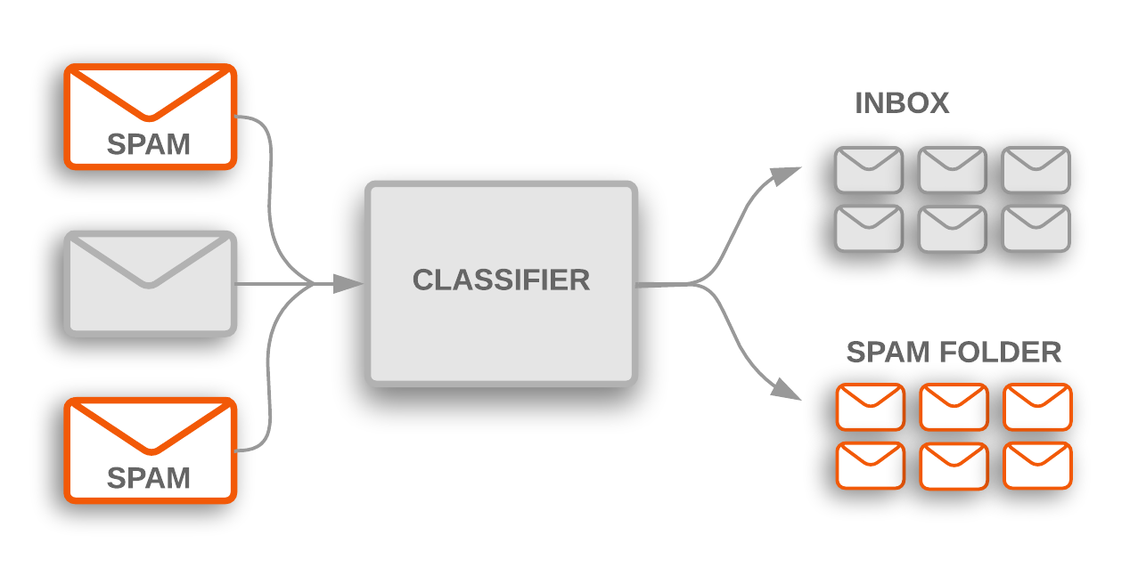
In that setting, the classes are usually spam and ham (because Spam is not ham). If an email contains words like won or prize, the classifier may assign a higher probability to the spam class because those words tend to appear there more often in the training data.

That basic idea is well known. The more interesting question is what happens when we apply it somewhere less obvious.

Could we use Naive Bayes to guess the author of an anonymous message?

That is the core idea behind stylometry: identifying an author from the statistical fingerprints in their writing.

Instead of asking whether a message looks like spam or ham, we ask whether it looks more like one writer than another.

This project is a Go implementation of a simple authorship classifier. It is a small but satisfying example of how far you can get with a mathematically simple model, some text preprocessing, and a carefully prepared corpus.

From Spam Classification to Authorship Attribution

At a high level, this project uses Naive Bayes in exactly the same way as a spam filter. The model takes a piece of text, considers a set of possible classes, and asks which class is the most likely source of that text.

In spam detection, those classes are spam and ham. In this project, the classes are the candidate authors themselves. Given a comment, the model no longer asks “Is this spam?” but instead “Which author does this comment look most like?”

That sounds almost too simple, but it works surprisingly well as long as different authors leave behind different statistical patterns in their writing.

Some people reuse the same words. Some overuse punctuation. Some write in shorter bursts, while others prefer long, winding sentences. None of these habits proves authorship on its own, but taken together they can form a recognizable fingerprint.

This is exactly where stylometry becomes a classification problem. If we can turn those writing habits into measurable features, Naive Bayes can estimate which author is most likely to have produced a given comment.

Constructing the Corpus

Of course, none of this works without data. Before I could train a classifier, I first needed a corpus of comments with known authorship.

To build it, I used a small Scrapy spider that crawled forum pages, followed pagination, and extracted individual comments together with the visible author name. For each comment, I stored three fields: the original text, the author label, and a lightly normalized version of the text that would later be used during training.

That normalization step was intentionally modest. I unescaped HTML entities, removed @ mentions, and collapsed repeated whitespace into single spaces.

The goal was not to aggressively clean the text (I’ll explain why in the next section), but simply to remove a bit of noise while preserving the stylistic patterns that might still carry authorship signal.

After collection, I anonymized the two writers as Author A and Author B and split the dataset into comment_sets/authorship_train.jsonl and comment_sets/authorship_validation.jsonl.

The training set contains 2195 comments in total: 1043 from Author A and 1152 from Author B. The validation set contains 1098 comments: 533 from Author A and 565 from Author B.

That split gives the model enough data to learn recurring patterns from each author while still leaving aside a separate set of unseen comments for evaluation. Once the corpus is in place, the next step is to turn those comments into something the model can actually count.

import scrapy
from scrapy import Request


class MakeCorpus(scrapy.Spider):
    def __init__(self, *args, **kwargs):
        super().__init__(*args, **kwargs)
        self.seen_pages = set()

    def start_requests(self):
        for url in self.start_urls:
            yield Request(url, callback=self.parse, dont_filter=True)

    def normalize_text(self, text):
        normalized = html.unescape(text).replace("@", "")
        return re.sub(r"\s+", " ", normalized).strip()

    def parse(self, response):
        if response.url in self.seen_pages:
            return

        self.seen_pages.add(response.url)

        for comment in response.css("div.comment"):
            author = comment.css("div.comment-title a::text").get()
            comment_text = " ".join(
                text.strip()
                for text in comment.xpath(
                    './div[contains(@class, "comment-content")]//text()[not(ancestor::span[contains(translate(@style, " ", ""), "color:silver")])]'
                ).getall()
                if text.strip()
            )

            if not author or not comment_text.strip():
                continue

            comment_text = html.unescape(comment_text.strip())

            yield {
                "author": author.strip(),
                "comment_text": comment_text,
                "comment_text_normalized": self.normalize_text(comment_text),
                "page_url": response.url,
            }

        pagination_hrefs = response.css("ul.pagination a.page-link::attr(href)").getall()
        page_numbers = []
        for href in pagination_hrefs:
            if not href:
                continue
            tail = href.rsplit("forum.", 1)[-1].rsplit(".html", 1)[0]
            if tail.isdigit():
                page_numbers.append(int(tail))

        max_page = max(page_numbers, default=1)
        for page_number in range(2, max_page + 1):
            page_url = f"{url}.{page_number}.html"
            if page_url not in self.seen_pages:
                yield Request(page_url, callback=self.parse)

Bag of Words and a Very Imperfect Tokenizer

The simplest way to do that is with a Bag of Words model.

Instead of treating a comment as a carefully structured sentence, we treat it as a collection of tokens and count how often those tokens appear.

Word order is discarded; what matters is which words, symbols, and fragments show up, and how often they do so for each author.

That representation is crude, but it fits Naive Bayes very well.

The model does not need a deep understanding of grammar or meaning. It only needs a consistent way to count features and compare how strongly they are associated with one author versus another.

My tokenizer is, frankly, pretty bad.

It removes URLs, splits text into groups of letters and numbers, preserves punctuation and symbol clusters, and converts everything to uppercase.

That is enough to produce tokens, but it is nowhere near linguistically sophisticated.

It does not understand morphology, syntax, or the fact that many surface forms may really belong to the same underlying word.

Two common ways to improve this are stemming and lemmatization.

Stemming reduces a word to a rough root by chopping off endings, often with fairly mechanical rules.

Lemmatization goes a step further and tries to recover the dictionary form of a word based on actual linguistic analysis.

In English, that might mean mapping running to run.

In Slovene, where words inflect heavily for case, number, gender, and other grammatical categories, that kind of normalization becomes much more important.

This is exactly why the tokenizer is especially weak for Slovene. A single word can appear in many different forms, and without stemming or lemmatization the model treats each of those forms as a separate token.

That fragments the data, increases sparsity, and makes it harder for the classifier to learn that several related forms really belong together.

And yet, for stylometry, this weakness is not entirely a disaster.

Authorship attribution is also about habits. Inflected forms, punctuation choices, repeated expressions, emphatic capitalization, odd symbol usage, and other messy surface details can all carry stylistic signal. So while this tokenizer is undeniably crude, it also preserves a surprising amount of the texture of how someone writes.

In other words, it is bad at linguistic normalization, but not necessarily bad at preserving authorial fingerprints. For this project, that turns out to be good enough.

Without further ado, here is our very simplistic tokenizer and normalizer:

func tokenize(text string) []string {
	// 1. Strip URLs
	var urlRe = regexp.MustCompile(`(?i)\b(?:https?://|www\.)\S+\b`)
	cleaned := urlRe.ReplaceAllString(text, "")

	// 2. Match words/numbers OR match symbols/emojis/punctuation
	var wordRe = regexp.MustCompile(`[\p{L}\p{N}]+|[^\p{L}\p{N}\s]+`)
	matches := wordRe.FindAllString(cleaned, -1)

	// 3. Uppercase
	var tokens []string
	for _, match := range matches {
		tokens = append(tokens, strings.ToUpper(match))
	}
	return tokens
}

Training the Model

Once the corpus has been collected and each comment has been turned into tokens, the training step is almost disappointingly simple.

There is no gradient descent, no backpropagation, and no expensive optimization loop (If you’re interested in this I highly recommend Neural Networks: Zero to Hero). The model just counts.

For every comment in the training set, we already know the correct author. That means we can walk through the tokens in that comment and update a few statistics that will later be enough for classification.

The first and most important one is AuthorTokenCounts.

This is a nested map that stores how many times each token was seen for each author. If Author A uses some word, phrase fragment, or punctuation pattern more often than Author B, that difference will start to show up here.

The model also keeps track of AuthorTotalTokens, which stores the total number of tokens observed for each author, and DocCounts, which stores how many training comments belong to each author.

Finally, it builds Vocab, the set of all unique tokens seen during training, and increments TotalDocs, the total number of documents in the corpus.

Taken together, these counts form the statistical memory of the classifier.

The training phase does not make predictions yet. It simply builds the frequency tables that will later let us estimate things like how likely is this token under Author A? and how common is Author B overall?

In code, that entire process fits into a single compact function:

type Model struct {
	AuthorTokenCounts map[string]map[string]int
	AuthorTotalTokens map[string]int
	DocCounts         map[string]int
	Vocab             map[string]struct{}
	TotalDocs         int
}

type Comment struct {
	Author                string `json:"author"`
	CommentText           string `json:"comment_text"`
	CommentTextNormalized string `json:"comment_text_normalized"`
}

func (m *Model) Train(comments []Comment) {
	for _, comment := range comments {
		author := comment.Author
		if author == "" {
			continue
		}

		if m.AuthorTokenCounts[author] == nil {
			m.AuthorTokenCounts[author] = map[string]int{}
		}

		m.DocCounts[author]++
		m.TotalDocs++

		for _, token := range tokenize(comment.CommentTextNormalized) {
			m.AuthorTokenCounts[author][token]++
			m.AuthorTotalTokens[author]++
			m.Vocab[token] = struct{}{}
		}
	}

}

This is one of the nicest things about Naive Bayes: once the data is prepared, “training” is really just counting the right things.

The mathematics only comes later, when we use those counts to score an unseen comment.

A Short Math Interlude

Now that the counting machinery is in place, we can finally write down the actual Naive Bayes formula:

P(A | B) = P(B | A) * P(A) P(B)

This looks more intimidating than it really is. The formula simply says: given some observed evidence B, what is the probability that hypothesis A is true?

Here is what each term means:

P(A | B) is the posterior: the probability that hypothesis A is true after we have seen evidence B
P(A) is the prior: how plausible A was before looking at the evidence
P(B | A) is the likelihood: how probable the evidence B would be if A were true
P(B) is the evidence: the overall probability of observing B

In a spam filter, A might be the hypothesis “this email is spam”, and B might be the words in that email. In our case, A is the hypothesis that a particular author wrote the comment, and B is the tokenized comment itself.

So for stylometry, the formula becomes:

P(Author | Comment) = P(Comment | Author) * P(Author) P(Comment)

Read in plain English, this asks: what is the probability that a given author wrote this comment, given the words and symbols that appear inside it?

The prior, P(Author), comes from how often that author appears in the training set. The likelihood, P(Comment | Author), comes from the token frequencies we counted during training. And the denominator, P(Comment), serves as a normalizing constant that makes the final probabilities add up nicely across all candidate authors.

Of course, a full comment is not a single observation but a sequence of many tokens.

That is where the “naive” part comes in: Naive Bayes assumes that, once we know the author, the tokens are conditionally independent of one another.

That assumption is obviously false in real language, but it makes the model simple, fast, and surprisingly effective.

Under that assumption, we can rewrite the likelihood of a whole comment as a product of per-token probabilities:

P(C | A) = P(t₁ | A) · P(t₂ | A) · P(t₃ | A) · ...

Here, C stands for the whole comment and t₁, t₂, t₃, … are the individual tokens inside it. This is the core naive assumption in its most explicit form: once we condition on the author A, we treat the tokens as independent pieces of evidence.

The denominator can also be written out more explicitly:

P(C) = P(C | A₁) · P(A₁) + P(C | A₂) · P(A₂) + P(C | A₃) · P(A₃) + ...

This is really just the law of total probability. To get the overall probability of seeing comment C, we sum over all possible authors: the probability of seeing C if A₁ wrote it, weighted by how likely A₁ is; plus the same quantity for A₂, A₃, and so on.

So the real task becomes estimating how likely each token is under each author, combining those probabilities, and then comparing the resulting scores. That is exactly what the next part of the implementation does.

Turning the Formula into Code

At the implementation level, this means looping over all candidate authors and computing three things:

the prior P(Author)
the likelihood contribution of each token P(token | Author)
the final posterior score for that author

The code below follows that structure directly. For each author, it starts with the prior, then walks through the tokens in the comment and adds the contribution of each one. Tokens that were never seen during training are skipped, and token probabilities are smoothed so that unseen author-token combinations do not collapse the whole score to zero.

type AuthorScore struct {
	Author      string
	Probability float64
}

func (a AuthorScore) String() string {
	return fmt.Sprintf("Author: %s, Probability: %f\n", a.Author, a.Probability)
}

type AuthorScores []AuthorScore

func (a AuthorScores) String() string {
	sb := strings.Builder{}
	for i, score := range a {
		sb.WriteString(fmt.Sprintf("%d. %2.2f%% probability it's author '%s'\n", i+1, score.Probability*100, score.Author))
	}
	return sb.String()
}

func (m *Model) GetSortedProbabilities(comment string) AuthorScores {
	// ── Naive Bayes classifier ────────────────────────────────────────────────
	// Goal: find P(Author | Comment) for every known author.
	//
	// Bayes' theorem:
	//
	//   P(A | C) = P(C | A) · P(A)
	//              ───────────────
	//                   P(C)
	//
	// Where:
	//   P(A | C)  — posterior:   probability this author wrote the comment
	//   P(A)      — prior:       base rate of seeing this author in training data
	//   P(C | A)  — likelihood:  probability the comment's tokens were produced by author A
	//   P(C)      — evidence:    normalising constant (same for all authors, so
	//                            used only to turn log-scores into probabilities)
	//
	// "Naive" assumption: tokens are conditionally independent given the author,
	// so the joint likelihood factorises into a product of per-token likelihoods:
	//
	//   P(C | A) = ∏  P(tᵢ | A)
	//               i
	//
	// Working in log-space turns that product into a sum, avoiding float underflow:
	//
	//   log P(A | C) ∝  log P(A)  +  Σ log P(tᵢ | A)
	// ─────────────────────────────────────────────────────────────────────────

	vocabSize := len(m.Vocab)
	tokens := tokenize(comment)

	// Stores  log[ P(A) · P(C|A) ]  for every author — the un-normalised log posterior.
	logNumerators := make(map[string]float64)
	maxScore := math.Inf(-1)

	for author, docCount := range m.DocCounts {

		// ── Prior:  log P(A) ─────────────────────────────────────────────────
		// Maximum-likelihood estimate from training-corpus frequencies:
		//   P(A) = (number of documents by A) / (total documents)
		score := math.Log(float64(docCount) / float64(m.TotalDocs))

		totalTokens := m.AuthorTotalTokens[author]

		// ── Laplace (add-1) smoothing denominator ────────────────────────────
		// Without smoothing, any token never seen for author A gives P(tᵢ|A) = 0,
		// which collapses the entire product to 0.
		// Add-1 smoothing pretends every token in the vocabulary was seen at
		// least once, giving a safe non-zero floor:
		//
		//   P(tᵢ | A) = (count(tᵢ, A) + 1) / (totalTokens(A) + |Vocab|)
		//                                      ──────────────────────────
		//                                           this denominator
		denominator := float64(totalTokens + vocabSize)

		for _, token := range tokens {
			// ── Out-of-vocabulary (OOV) guard ────────────────────────────────
			// Tokens completely absent from the training vocabulary carry no
			// discriminative signal for any author; skip them uniformly so they
			// don't artificially penalise every author equally.
			if _, exists := m.Vocab[token]; !exists {
				continue
			}

			// ── Likelihood (per token):  log P(tᵢ | A) ──────────────────────
			// Laplace-smoothed token probability for this author:
			//   numerator   = count(tᵢ, A) + 1   (the +1 is the Laplace pseudocount)
			//   denominator = totalTokens(A) + |Vocab|
			count := m.AuthorTokenCounts[author][token]
			prob := float64(count+1) / denominator

			// Accumulate into the log posterior sum:
			//   log P(A|C) ∝ log P(A) + Σ log P(tᵢ|A)
			score += math.Log(prob)
		}

		// Un-normalised log posterior for this author: log[ P(A) · P(C|A) ]
		logNumerators[author] = score

		// Track the highest log-score for the numerical stabilisation step below.
		if score > maxScore {
			maxScore = score
		}
	}

	// ── Evidence (normalising constant):  log P(C) ───────────────────────────
	// P(C) = Σ_A  P(A) · P(C|A)   (law of total probability)
	//
	// In log-space that sum cannot be computed directly. The log-sum-exp trick
	// subtracts the maximum log-score before exponentiating, keeping values in a
	// numerically safe range and avoiding both overflow and underflow:
	//
	//   log P(C) = maxScore + log( Σ_A exp(logNumerator_A − maxScore) )
	sumExp := 0.0
	for _, score := range logNumerators {
		sumExp += math.Exp(score - maxScore)
	}
	logPC := maxScore + math.Log(sumExp)

	// ── Posterior:  P(A | C) for every author ────────────────────────────────
	// Apply Bayes' theorem by subtracting the log evidence from each log numerator:
	//
	//   log P(A | C) = log[ P(A) · P(C|A) ] − log P(C)
	//   P(A | C)     = exp( log P(A|C) )
	//
	// The results are guaranteed to be in [0, 1] and sum to 1 across all authors.
	var results AuthorScores
	for author, score := range logNumerators {
		logConfidence := score - logPC        // log posterior
		confidence := math.Exp(logConfidence) // posterior probability

		results = append(results, AuthorScore{
			Author:      author,
			Probability: confidence,
		})
	}

	// Return authors ranked by posterior probability — highest (most likely) first.
	sort.Slice(results, func(i, j int) bool {
		return results[i].Probability > results[j].Probability
	})

	return results
}

There are two details worth calling out here.

First, the code uses Laplace smoothing (Also known as Additive smoothing):

P(token | Author) = count(token, Author) + 1 totalTokens(Author) + |Vocab|

Without that +1, any token never seen for a given author would get probability zero, and since the full likelihood is a product, one zero would wipe out the entire score.

Second, the code does not multiply raw probabilities directly. It works in log-space instead. That deserves its own explanation.

The Log-Sum-Exp Trick

Let us start with something almost embarrassingly simple:

e^(-1) = 1 e

e^(-2) = 1 e^2

e^(-10) = 1 e^10

So a negative exponent is just another way of writing a fraction. The more negative the exponent, the smaller the number becomes.

That is useful because probabilities are often small fractions. For example, if a token probability is 1/100, its logarithm is negative. And if we exponentiate that log value, we get the original fraction back.

Now imagine multiplying many such fractions together:

P(C | A) = 120 * 150 * 1100 * 140 * ...

After enough tokens, that product becomes extremely small. Mathematically, that is fine.

Computationally, it is a problem: a floating-point number may underflow toward zero simply because the computer cannot represent something that tiny accurately.

The standard fix is to take logarithms. Logarithms turn products into sums:

log(a * b * c) = log(a) + log(b) + log(c)

So instead of computing:

P(C | A) = P(t₁ | A) * P(t₂ | A) * P(t₃ | A) * ...

we compute:

log P(C | A) = log P(t₁ | A) + log P(t₂ | A) + log P(t₃ | A) + ...

And once we include the prior, the numerator becomes:

log(P(C | A) * P(A)) = log P(A) + log P(t₁ | A) + log P(t₂ | A) + ...

This is much safer numerically. Adding a bunch of negative numbers is much less dangerous than multiplying a bunch of tiny fractions.

But now we hit a subtle problem.

The numerator is easy in log-space because it is a product. The denominator, P(C), is not a product. It is a sum over authors:

P(C) = P(C | A₁) * P(A₁) + P(C | A₂) * P(A₂) + P(C | A₃) * P(A₃) + ...

So if we define:

s₁ = log(P(C | A₁) * P(A₁))
s₂ = log(P(C | A₂) * P(A₂))
s₃ = log(P(C | A₃) * P(A₃))

then the denominator becomes:

P(C) = e^(s₁) + e^(s₂) + e^(s₃) + ...

and therefore:

log P(C) = log(e^(s₁) + e^(s₂) + e^(s₃) + ...)

That is the source of the name log-sum-exp: we are taking a log of a sum of exp terms.

The problem is that some of the sᵢ values may be very negative. In that case, e^(sᵢ) becomes an absurdly tiny fraction. Or one score may be much larger than the others, and exponentiating everything directly becomes numerically unstable.

The trick is to factor out the largest score. Let:

m = max(s₁, s₂, s₃, ...)

Then:

e^(s₁) + e^(s₂) + e^(s₃) + ...
= e^m * (e^(s₁ - m) + e^(s₂ - m) + e^(s₃ - m) + ...)

Taking the logarithm of both sides gives:

log P(C) = m + log(e^(s₁ - m) + e^(s₂ - m) + e^(s₃ - m) + ...)

This is much more stable, because now the largest exponent is e^0 = 1, and all the others are less than or equal to 1. Instead of dealing with huge or tiny exponentials, we normalize everything around the biggest score.

That is exactly what this part of the code is doing:

sumExp := 0.0
for _, score := range logNumerators {
	sumExp += math.Exp(score - maxScore)
}
logPC := maxScore + math.Log(sumExp)

Once we have logPC, we subtract it from each author’s log-score and exponentiate one last time.

That gives us proper posterior probabilities that sum to 1.

Evaluation

Once the model is trained, the most important question is simple: does it actually identify the correct author on unseen comments?

To answer that, I evaluate the classifier on the separate validation set rather than on the training data. This matters because doing well on comments the model has already seen would not tell us much. The real test is whether the learned token patterns generalize to new comments.

The evaluation procedure is straightforward. For each comment in comment_sets/authorship_validation.jsonl, the model computes posterior probabilities for all candidate authors, sorts them, and takes the top prediction. If the most likely author matches the ground-truth label, the prediction counts as correct.

In other words, this is a simple top-1 accuracy evaluation:

accuracy = correct predictions / total predictions

The code for that looks like this:

const probabilityThreshold = 0.80

func (m *Model) evaluate(comments []Comment) (int, int, int) {
	correct, wrong := 0, 0
	for _, comment := range comments {
		if pa := m.GetSortedProbabilities(comment.CommentTextNormalized)[0]; pa.Author == comment.Author {
			if pa.Probability < probabilityThreshold {
				log.Printf("Warning, low probability for %s: %2.2f", comment.Author, pa.Probability*100)
			}
			correct++
		} else {
			log.Printf("WRONG: true=%s predicted=%s prob=%.2f | %s",
				comment.Author, pa.Author, pa.Probability*100, comment.CommentText)
			wrong++
		}
	}
	return correct, len(comments), wrong
}

There are two useful ideas in this function.

First, it keeps the evaluation honest by using only the held-out validation set. Second, it does not just record whether a prediction was right or wrong; it also inspects the model’s confidence. If the predicted author is correct but the posterior probability is below 0.80, the code emits a warning. That is a useful reminder that correctness and confidence are not the same thing.

This kind of evaluation is still fairly minimal. It gives us a clear first signal about whether the model works, but it does not yet tell us everything. For example, it does not analyze which kinds of comments are hardest to classify, whether some stylistic features are more informative than others, or how sensitive the results are to the train-validation split.

Still, for a compact stylometry experiment, it is a good final checkpoint: train on one set of comments, test on another, and measure how often the most probable author is actually the right one.

So with this in mind, how does the model actually perform?

Eh, not great, not terrible…

Under optimal conditions, with only 2 authors (classes), with widely distinct writing styles, I managed to get 93.38% accuracy

go run main.go 

Training documents: 2195
Validation documents: 1098
Vocabulary size: 13985
Author: Author A | train docs: 1043 | train tokens: 29403
Author: Author B | train docs: 1152 | train tokens: 43428
Accuracy: 93.35% (1025/1098)
Wrong count: 73

Conclusion

For such a small and crude model, that result is honestly pretty encouraging, I think.

There is something satisfying about getting decent authorship predictions out of nothing more than token counts, Bayes’ theorem, Laplace smoothing, and a bit of care around numerical stability.

At the same time, it is important not to overstate what this number means.

This experiment is very much a best-case scenario. The model only has to choose between two authors, both represented by a reasonable amount of training data, and both distinct enough that their habits leave behind a detectable statistical signal. In that setting, even a rough Bag of Words approach can look surprisingly competent.

But if we started adding more authors, the seemingly decent accuracy would likely break down rather quickly.

There are several reasons for that.

First, the classification problem becomes intrinsically harder. With two authors, the model only has to decide between Author A and Author B. With ten or twenty authors, many more candidates may share similar vocabulary, punctuation habits, or topic preferences, and the decision boundary becomes much less clear.

Second, the weaknesses of the tokenizer would start to hurt more. Slovene morphology already fragments the vocabulary heavily, and without stemming or lemmatization many related word forms are treated as entirely separate tokens. With only two authors, the model can sometimes get away with this. With many authors, that sparsity becomes much more damaging.

And finally, Naive Bayes itself is a deliberately naive model. It ignores word order, treats tokens as conditionally independent, and cannot capture higher-level stylistic structure very well. That simplicity is part of its charm, but it also places a ceiling on how far the method can scale.

So I do not mean to say this as a serious forensic authorship system. I would treat it as a neat demonstration that even a mathematically simple classifier can recover real stylistic signal from text.

That, to me, is the most interesting takeaway from the whole project: not that Naive Bayes solved stylometry, but that stylometric fingerprints are strong enough to show up even through a very imperfect pipeline.

Appendices

If you’re interested in source code for whatever reason it is available here. It also includes train and validation sets.

Stylometry with Naive Bayes in Go